Contents
Training a language model to use tools can look like a large jump from training it to solve math problems. The model now has to search, inspect results, choose an action, and deal with whatever happens next. Coming from math RLVR, I found that much of the learning algorithm carried over. What felt less familiar was the environment around it.
This post collects what I learned while making that transition. I start with the token-level MDP behind math RLVR, replace a completion with an interactive trajectory, and follow the consequences for credit assignment and rollout collection. A shopping task serves as a running example. It is simple enough to keep the mechanics visible, but already exposes problems that also arise in browser, coding, and simulator agents.
The convenient environment behind math RLVR
Consider a prompt \(x\) and a sampled solution \(y=(y_1,\ldots,y_T)\). A verifier assigns the completed solution a reward \(R(x,y)\), often a binary correctness label. We can describe generation as an MDP by taking the state to be the prompt and generated prefix, and the action to be the next token:
Given a token, the transition is deterministic: append it to the prefix. Resetting the environment means returning to the prompt. Rollouts can be generated in parallel without maintaining a separate browser or simulator for each sample. When the verifier is reliable, we also get an inexpensive reward without training a reward model. These are substantial conveniences, even though the underlying optimization problem can still be difficult.
In the familiar outcome-reward version of GRPO, we sample \(G\) solutions from a frozen policy \(\pi_{\mathrm{old}}\), score them, and normalize their rewards within the group. Writing \(\mu_R\) and \(\sigma_R\) for the group mean and standard deviation gives
Ignoring normalization factors and an optional KL penalty, the clipped policy loss has the form
The same advantage \(\hat A_i\) is applied to every generated token in solution \(i\). The verifier does not identify which reasoning steps were useful; it only judges the result. A correct answer can therefore reinforce a completion containing a detour or an incorrect intermediate step. Keep this limitation in mind when we move to agents.
From a completion to an interaction
Suppose the task is to find a red hiking backpack under $80 with at least a four-star rating. In a shopping simulator, the agent might search for backpacks, open a product page, select a color, and submit a purchase. Each action produces information that was unavailable when the previous action was generated:
User: Find a red hiking backpack under $80, rated at least four stars.
Agent: search["red hiking backpack"]
Environment: Search results …
Agent: click["item_3"]
Environment: Price: $69. Rating: 4.5. Available colors: red, blue.
Agent: select["red"]
Environment: Red selected. Price: $69.
Agent: buy["item_3"]
Now a rollout is an alternating sequence of observations and actions, \(\tau=(o_0,a_0,o_1,a_1,\ldots,o_T)\). The policy acts on the interaction history \(h_t=(o_0,a_0,\ldots,o_t)\), and the environment supplies the next observation:
There are two transitions to account for. Tokens extend the current action prefix; a completed action is then executed in the environment. The latter may involve hidden state, stochastic outcomes, and external latency. Even a deterministic simulator requires maintaining and advancing an environment instance for each rollout.
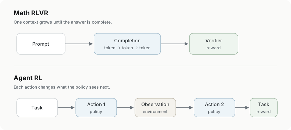
It helps to distinguish the true environment state \(s_t^{\mathrm{env}}\), the observable history \(h_t\), and the context \(c_t=f(h_t)\) actually passed to the model. An agent may see only part of a webpage or a summary of earlier turns. Its policy is then \(\pi_\theta(a_t\mid c_t)\). Below, state-value notation refers to the history unless stated otherwise; a shortened context need not retain all the information needed to predict what happens next.
The first implementation of agent GRPO can otherwise be quite familiar. Sample several complete trajectories for the same task, compute their terminal rewards, and assign a group-relative advantage to each trajectory. The main change in the loss is a mask: user messages and environment outputs provide context, but only policy-generated tokens receive policy-gradient loss.
The probability ratio must use the context available when that token was sampled. Flattening the transcript is convenient when the model retains the full history. If the rollout system truncates or summarizes context between turns, training must reproduce those contexts. Feeding a reconstructed full history would evaluate a different conditional probability.
What did the successful agent do right?
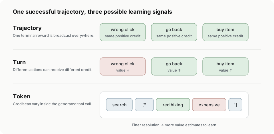
Imagine that our agent first opens the wrong backpack, notices that it costs too much, goes back, and finds a suitable one. The episode succeeds. With a positive trajectory-level advantage, the update encourages all of its generated actions, including the mistaken click. It also encourages the recovery, which was useful given the mistake. A single terminal label cannot distinguish the two.
This is the same credit-assignment issue we encountered in math RLVR, but the action structure makes it more visible. A trajectory may contain dozens of tool calls, repeated searches, invalid actions, and repairs. We would like to know whether a particular decision improved the agent’s prospects, rather than only whether the episode eventually succeeded.
For an undiscounted task with a binary terminal reward, a value function has a direct interpretation:
If the estimated value rises from 0.2 to 0.7 after opening a product page, that transition looks promising. The estimate is still policy-dependent: a useful page only helps if the agent can make good decisions from it. With intermediate rewards or discounting, the value instead estimates the remaining discounted return. The corresponding temporal-difference residual and GAE advantage are
For a true terminal state, the bootstrap value is zero. Before termination, a critic supplies a local learning signal even when intermediate rewards are absent. That signal is only as useful as the critic: an increase in a learned value is an estimate of progress, not an independent verification that the action was good.
An agent turn is itself a token sequence, \(a_t=(w_{t,1},\ldots,w_{t,L_t})\). One implementation broadcasts the turn advantage \(\hat A_t\) to its tokens and applies the clipped loss using token probability ratios. This gives different turns different credit while preserving the LM training interface. Clipping individual token ratios is a modeling choice; it is not identical to clipping the probability ratio of the entire action, which is a product of token ratios.
Values at the action and token levels
A state value averages over the actions the policy might take. An action value instead conditions on a particular choice. Returning to the undiscounted terminal-reward setting,
This is the comparison we wanted for the mistaken click: how does this action compare with what the policy would typically do from the same history? A conceptually straightforward way to estimate it is to execute the action and sample several independent continuations under the policy:
Six successes among eight continuations give an estimate of 0.75. The arithmetic is easy; obtaining the samples is expensive. Eight continuations from each of 20 decision points means 160 additional rollouts, each with its own remaining model calls and environment steps. In a stochastic environment, the continuations also need to capture the possible outcomes of the action, rather than all sharing a single favorable outcome.
We can apply the same reasoning inside an action. Before token \(j\), the expanded state is \((h_t,w_{t,<j})\). After choosing that token, the remaining randomness includes both the rest of the tool call and everything that follows its execution:
For the backpack task, a value model might judge the prefix search["cheap more promising than search["expensive. It is evaluating expected eventual success, including how the policy is likely to complete the prefix. It does not need to wait for an executable tool call, though estimating these values accurately is another learning problem.
Turn-level and token-level values thus describe different points in the same expanded process. At the final token of a fully specified action, their targets agree under matching conditioning and return conventions:
Monte Carlo branching is only one route to denser feedback. A process reward model can score useful searches, invalid actions, or repetition; an environment can expose intermediate completion signals; hindsight analysis can help distinguish an early useful action from a later failure. Each introduces assumptions about what deserves credit. Learned rewards can be exploited, and engineered progress rewards can change the objective if they reward behavior that does not ultimately help complete the task.
Exploration includes learning to recover
Sampling different math solutions explores different generated prefixes. Sampling agent actions also changes which external observations the model will encounter. Opening two different products creates two different opportunities for the next decision. Deleting a file or submitting a form may remove the possibility of returning to the previous state. Both the policy and the environment determine the resulting trajectory tree.
Recovery therefore deserves attention in its own right. After opening an unsuitable backpack, a competent agent should inspect the mismatch and go back. To learn that behavior, it needs experience in states reached through mistakes. Clean expert demonstrations may provide little coverage of those states, even when they show the shortest successful path through every training task.
This also makes the credit-assignment problem more subtle than penalizing every detour. We want to reduce avoidable mistakes while retaining the actions that repair them. A recovery action can have high value conditional on a bad state, even though a better policy would rarely enter that state in the first place.
The cost of collecting a trajectory
In math RLVR, collection is roughly a batch of model generations followed by verifier calls. For an agent, collection includes a persistent interaction loop. A minimal synchronous sketch looks like this; token IDs, behavior log probabilities, and masks are omitted to keep the control flow readable.
for task in batch:
    trajectories = []
    for _ in range(group_size):
        history = [env.reset(task)]
        trajectory = []
        done = False

        for turn in range(max_turns):
            action = policy.generate(history)
            next_obs, reward, done, info = env.step(action)
            trajectory.append(
                (history.copy(), action, reward, next_obs, done)
            )
            history = history + [action, next_obs]
            if done:
                break

        trajectories.append({
            "steps": trajectory,
            "truncated": not done,
        })

    update_policy(trajectories)
The actual buffer must preserve enough information to reconstruct the training conditionals: generated tokens, policy-token masks, behavior-policy log probabilities, the contexts shown to the model, rewards, and termination status. A critic may also require value predictions. Environment state identifiers or snapshots are useful when a trajectory will later be replayed or branched.
Termination deserves care. Success, task failure, and a collection timeout are different events. If collection stops at a time limit while the underlying task could continue, value estimation may need to bootstrap from the last state. If the task itself defines exceeding the turn budget as failure, that is a terminal outcome. Treating both cases identically can distort the critic’s targets.
At scale, a rollout manager distributes tasks to policy and environment workers. Their trajectories enter a buffer, reward and value computation produce advantages, and a learner updates the policy. New weights then return to the rollout workers. The data flow is straightforward; keeping every stage supplied with useful work is harder.
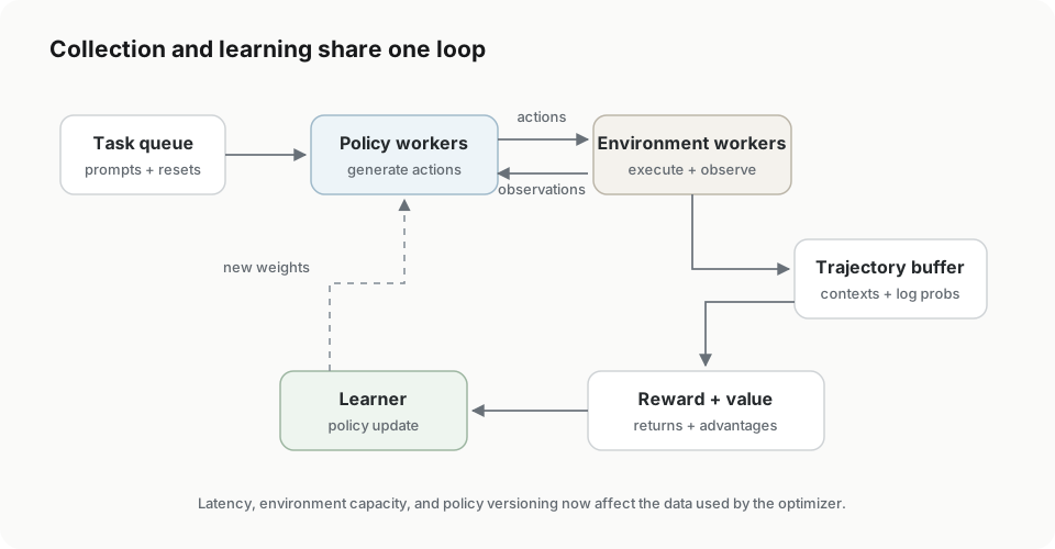
Suppose each turn takes two seconds of model inference and one second of environment interaction. A 20-turn episode takes about a minute, and a GRPO group of 16 episodes requires 320 model–environment interactions. Parallelism reduces wall-clock time, but it still requires enough independent environments and inference capacity. Resetting a browser, serializing simulator state, or waiting for a tool can become a substantial part of collection cost.
Branching adds a further requirement. To compare actions from the same point, the system must restore the environment as well as the model context. Without snapshots, each branch may require replaying the prefix, which is costly and may fail to reproduce the same state in a stochastic environment. LM prefix caching and environment checkpointing address different parts of this cost. Their availability can determine whether a proposed Q estimator is practical at all.
Throughput and policy freshness
The simplest training schedule freezes \(\pi_{\theta_k}\), collects a batch of trajectories, updates to \(\theta_{k+1}\), and repeats. This keeps the behavior policy well defined and the data recent. It also makes the learner wait for slow episodes, while faster workers may sit idle.
Asynchronous collection lets workers continue interacting while the learner updates. Better utilization comes with older data: a trajectory generated under version 100 might reach a learner already at version 110. Stored behavior-policy probabilities make it possible to form ratios such as
Those ratios do not make arbitrary policy lag harmless. Large distribution changes can make importance weights unreliable, and token-level PPO clipping does not fully correct the change in visited histories. A useful collection system needs to track policy versions and control how stale a trajectory can become before it is used.
Value learning offers a possible way to reuse more experience. Whereas PPO and GRPO policy updates generally rely on recent samples, a critic may be trained with replay. There is a qualification: \(V^\pi\) and \(Q^\pi\) depend on the continuation policy. A terminal outcome generated by an old policy is not automatically an unbiased target for the current one. Reusing old trajectories requires suitable off-policy targets or corrections, or accepting the resulting approximation. A larger buffer alone does not resolve that mismatch.
Using values without updating the model
A learned value can also guide action selection at inference time. For example, one could reweight a fixed base policy using
Here \(\beta\) controls the strength of the preference for higher-valued actions. Unlike a policy-gradient update, this leaves the base model’s parameters fixed and changes the distribution used to sample actions. A turn-level value can rerank complete candidate tool calls before execution; a token-level value can intervene while a candidate is still being generated. The latter offers finer control, but also requires useful value estimates at many more decision points.
The progression from math RLVR to agent RL is therefore a progression in the structure of experience. A terminal reward can supervise an entire interaction, a critic can distinguish individual turns, and a token-level value can distinguish choices within a turn. Finer credit is attractive when it separates useful behavior from mistakes, but it has to justify the cost and error introduced by estimating it.
When reading an agent RL paper, I find it useful to trace one trajectory all the way through the system: what the model sees, what it generates, what changes in the environment, where the reward comes from, and which generated tokens receive which advantage. Then ask how that trajectory was collected and how old its policy is by the time training uses it. These details often explain more about the method’s behavior than the name of its optimizer.